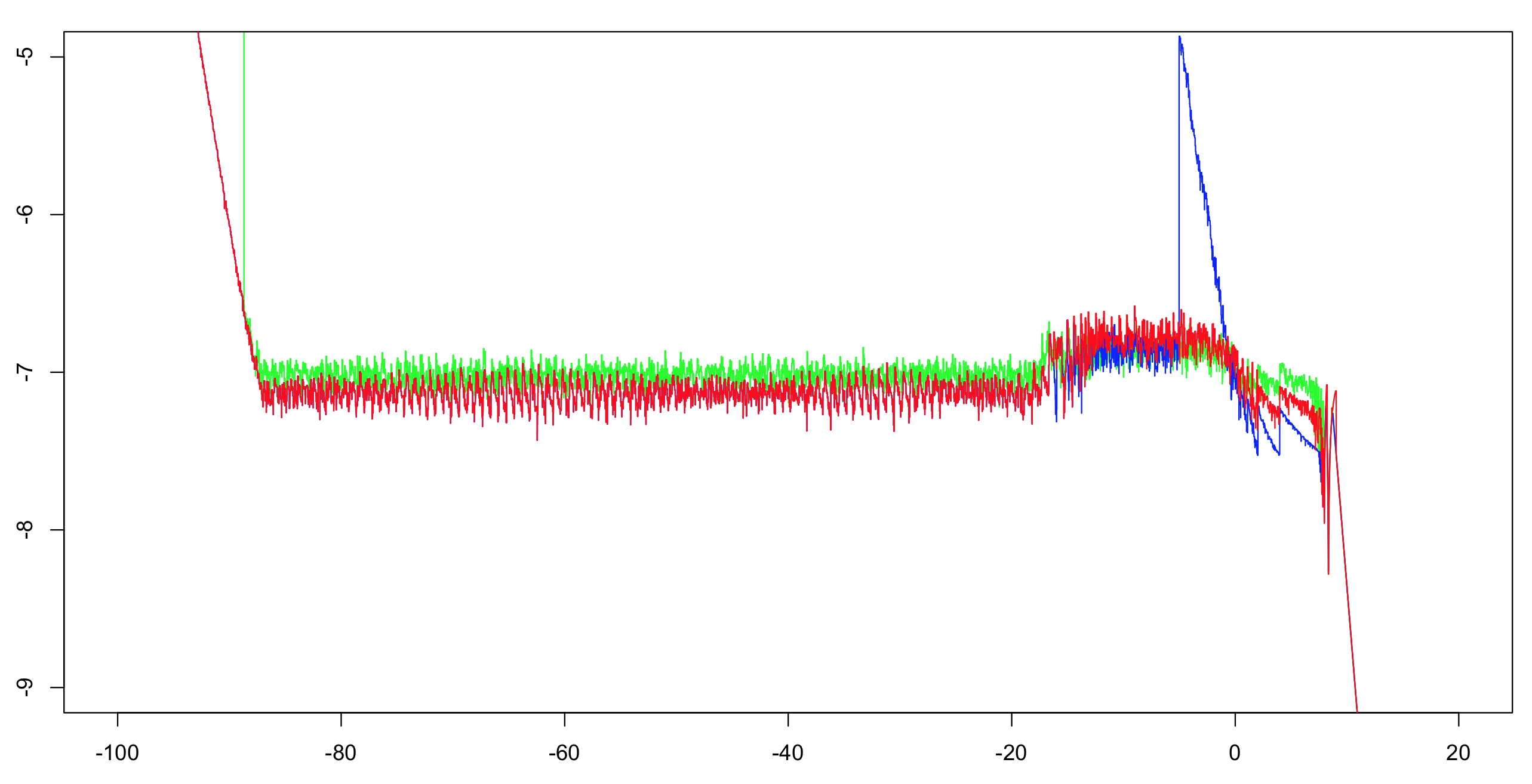
OP points to a particular implementation of the mish activation function for accuracy specifications, so I had to characterize this first. That implementation uses single precision (float), and is stable and accurate in the positive half-plane. In the negative half-plane, because it uses logf instead of log1pf, relative error quickly grows a $x\to-\infty$. Loss of accuracy starts around $-1$ and already at $-16.6355324$ the implementation falsely returns $0$, because $\exp(-16.6355324) = 2^{-24}$.
The same accuracy and behavior can be achieved by using a simple mathematical transformation that eliminates $\mathrm{tanh}$, and considering that GPUs typically offer a fused multiply-add (FMA) as well as a fast reciprocal, which one would want to utilize. Exemplary CUDA code looks as follows:
__device__ float my_mishf (float x)
{
    float r;
    float e = expf (x);
    r = 1.0f / fmaf (fmaf (-0.5f, e, -1.0f), e, -1.0f);
    r = fmaf (r, x, x);
    return r;
}
As with the reference implementation pointed to by OP, this has excellent accuracy in the positive half-plane, and in the negative half-plane error increases rapidly so at $-16.6355324$ the implementation falsely returns $0$.
If there is a desire to address these accuracy issues, we can apply the following observations. For sufficiently small $x$, $f(x) = x \exp(x)$ to within floating-point accuracy. For float computation this holds for $x < -15$. For the interval $[-15,-1]$, we can use a rational approximation $R(x)$ to compute $f(x) := R(x)x\exp(x)$. Exemplary CUDA code looks as follows:
__device__ float my_mishf (float x)
{
    float r;
    if (x >= -1.0f) {
        float e = expf (x);
        r = 1.0f / fmaf (fmaf (-0.5f, e, -1.0f), e, -1.0f);
        r = fmaf (r, x, x);
    } else {
        float eh = expf (0.5f * x);
        float p =        1.03628484e-3f;  //  0x1.0fa7e6p-10
        p = fmaf (p, x, -7.28869531e-3f); // -0x1.ddac04p-8
        p = fmaf (p, x,  3.47027816e-2f); //  0x1.1c4902p-5
        p = fmaf (p, x, -3.54762226e-1f); // -0x1.6b46cap-2
        p = fmaf (p, x,  8.58785570e-1f); //  0x1.b7b2bep-1
        p = fmaf (p, x, -1.38065982e+0f); // -0x1.6172ecp+0
        p = fmaf (p, x,  5.97694337e-1f); //  0x1.3204fep-1
        float q =        1.03527203e-3f;  //  0x1.0f63eep-10
        q = fmaf (q, x, -7.35638570e-3f); // -0x1.e21bacp-8
        q = fmaf (q, x,  3.28683928e-2f); //  0x1.0d4204p-5
        q = fmaf (q, x, -3.79927397e-1f); // -0x1.850bb0p-2
        q = fmaf (q, x,  6.86127126e-1f); //  0x1.5f4c0ep-1
        q = fmaf (q, x, -1.81509292e+0f); // -0x1.d0a9eep+0
        q = fmaf (q, x,  1.00000000e+0f); //  0x1.000000p+0
        r = (1.0f / q) * p;
        if (x < -15.0f) r = 1.0f;
        r = r * x * eh * eh;
    }
    return r;
}
Unfortunately, this accurate solution is achieved at the cost of a significant drop in performance. If one is willing to accept reduced accuracy while still achieving a smoothly decaying left tail, the following interpolation scheme, again based on $f(x) \approx x\exp(x)$, recovers much of the performance:
__device__ float my_mishf (float x)
{
    float r;
    float e = expf (x);
    if (x >= -6.0625f) {
        r = 1.0f / fmaf (fmaf (-0.5f, e, -1.0f), e, -1.0f);
        r = fmaf (r, x, x);
    } else {
        r = fmaf (-0.5f, e, 1.0f);
        r = r * x * e;
    }
    return r;
}
As a machine-specific performance enhancement, expf() could be replaced by the device intrinsic __expf().

