I was going through the text Introduction to Algorithm by Cormen et. al. where I came across an excerpt which I felt required a bit of clarification.
Now as far as I have learned that that while the Best Case and Worst Case time complexities of an algorithm arise for a certain physical input to the algorithm (say an input $A$ causes the worst case run time for an algorithm or say an input $B$ causes the best case run time of an algorithm , asymptotically), but there is no such physical input which causes the average case runtime of an algorithm as the average case run time of an algorithm is by it's definition the runtime of the algorithm averaged over all possible inputs. It is something I hope which only exists mathematically.
But on the other hand inputs to an algorithm which are neither the best case input nor the worst case input is supposed to be somewhere in between both the extremes and the performance of our algorithm is measured on them by none other than the average case time complexity as the average case time complexity of the algorithm is in between the worst and best case complexities just as our input between the two extremes.
Is it correct or incorrect to say that an input say $C$ causes an average run-time of an algorithm?
The excerpt from the text which made me ask such a question is as follows:
In context of the analysis of quicksort,
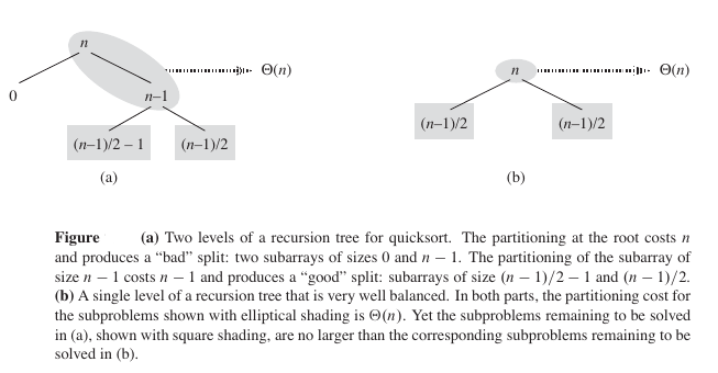
In the average case, PARTITION produces a mix of “good” and “bad” splits. In a recursion tree for an average-case execution of PARTITION, the good and bad splits are distributed randomly throughout the tree. Suppose, for the sake of intuition, that the good and bad splits alternate levels in the tree, and that the good splits are best-case splits and the bad splits are worst-case splits. Figure(a) shows the splits at two consecutive levels in the recursion tree. At the root of the tree, the cost is $n$ for partitioning, and the subarrays produced have sizes $n- 1$ and $0$: the worst case. At the next level, the subarray of size $n- 1$ undergoes best-case partitioning into subarrays of size $(n-1)/2 - 1$ and $(n-1)/2$ Let’s assume that the boundary-condition cost is $1$ for the subarray of size $0$.
The combination of the bad split followed by the good split produces three sub- arrays of sizes $0$, $(n-1)/2 - 1$ and $(n-1)/2$ at a combined partitioning cost of $\Theta(n)+\Theta(n-1)=\Theta(n)$. Certainly, this situation is no worse than that in Figure(b), namely a single level of partitioning that produces two subarrays of size $(n-1)/2$, at a cost of $\Theta(n)$. Yet this latter situation is balanced!

